In this project, we’ll classify images from the CIFAR-10 dataset. The dataset consists of airplanes, dogs, cats, and other objects. we’ll preprocess the images, then train a convolutional neural network on all the samples. The images need to be normalized and the labels need to be one-hot encoded. We’ll get to apply and build a convolutional, max pooling, dropout, and fully connected layers. At the end, We’ll get to see our neural network’s predictions on the sample images.
Get the Data
Run the following cell to download the CIFAR-10 dataset for python.
from urllib.request import urlretrieve
from os.path import isfile, isdir
from tqdm import tqdm
import problem_unittests as tests
import tarfile

cifar10_dataset_folder_path = 'cifar-10-batches-py'

# Use Floyd's cifar-10 dataset if present
floyd_cifar10_location = '/input/cifar-10/python.tar.gz'
if isfile(floyd_cifar10_location):
    tar_gz_path = floyd_cifar10_location
else:
    tar_gz_path = 'cifar-10-python.tar.gz'

class DLProgress(tqdm):
    last_block = 0

    def hook(self, block_num=1, block_size=1, total_size=None):
        self.total = total_size
        self.update((block_num - self.last_block) * block_size)
        self.last_block = block_num

if not isfile(tar_gz_path):
    with DLProgress(unit='B', unit_scale=True, miniters=1, desc='CIFAR-10 Dataset') as pbar:
        urlretrieve(
            'https://www.cs.toronto.edu/~kriz/cifar-10-python.tar.gz',
            tar_gz_path,
            pbar.hook)

if not isdir(cifar10_dataset_folder_path):
    with tarfile.open(tar_gz_path) as tar:
        tar.extractall()
        tar.close()


tests.test_folder_path(cifar10_dataset_folder_path)
CIFAR-10 Dataset: 171MB [24:05, 118KB/s]


All files found!
Explore the Data
The dataset is broken into batches to prevent our machine from running out of memory. The CIFAR-10 dataset consists of 5 batches, named data_batch_1, data_batch_2, etc.. Each batch contains the labels and images that are one of the following:
* airplane
* automobile
* bird
* cat
* deer
* dog
* frog
* horse
* ship
* truck
Understanding a dataset is part of making predictions on the data. Play around with the code cell below by changing the batch_id and sample_id. The batch_id is the id for a batch (1-5). The sample_id is the id for a image and label pair in the batch.
Ask yourself “What are all possible labels?”, “What is the range of values for the image data?”, “Are the labels in order or random?”. Answers to questions like these will help us preprocess the data and end up with better predictions.
%matplotlib inline
import helper
import numpy as np

# Explore the dataset
batch_id = 1
sample_id = 5
helper.display_stats(cifar10_dataset_folder_path, batch_id, sample_id)
Stats of batch 1:
Samples: 10000
Label Counts: {0: 1005, 1: 974, 2: 1032, 3: 1016, 4: 999, 5: 937, 6: 1030, 7: 1001, 8: 1025, 9: 981}
First 20 Labels: [6, 9, 9, 4, 1, 1, 2, 7, 8, 3, 4, 7, 7, 2, 9, 9, 9, 3, 2, 6]

Example of Image 5:
Image - Min Value: 0 Max Value: 252
Image - Shape: (32, 32, 3)
Label - Label Id: 1 Name: automobile

Implement Preprocess Functions
Normalize
In the cell below, implement the normalize function to take in image data, x, and return it as a normalized Numpy array. The values should be in the range of 0 to 1, inclusive. The return object should be the same shape as x.
def normalize(x):
    """
    Normalize a list of sample image data in the range of 0 to 1
    : x: List of image data.  The image shape is (32, 32, 3)
    : return: Numpy array of normalize data
    """
    #  Normalize Function
    return np.array((x - np.min(x)) / (np.max(x) - np.min(x)))
One-hot encode
Just like the previous code cell, we’ll be implementing a function for preprocessing. This time, we’ll implement the one_hot_encode function. The input, x, are a list of labels. Implement the function to return the list of labels as One-Hot encoded Numpy array. The possible values for labels are 0 to 9. The one-hot encoding function should return the same encoding for each value between each call to one_hot_encode. Make sure to save the map of encodings outside the function.
Hint: Don’t reinvent the wheel.
from sklearn.preprocessing import LabelBinarizer
lb_encoding = None

def one_hot_encode(x):
    """
    One hot encode a list of sample labels. Return a one-hot encoded vector for each label.
    : x: List of sample Labels
    : return: Numpy array of one-hot encoded labels
    """
    # Implement Function
    global lb_encoding

    if lb_encoding is not None:
        return lb_encoding.transform(x)
    else:
        lb = LabelBinarizer()
        lb_encoding = lb.fit(x)
    return lb_encoding.transform(x)
Randomize Data
As we saw from exploring the data above, the order of the samples are randomized. It doesn’t hurt to randomize it again, but we don’t need to for this dataset.
Preprocess all the data and save it
Running the code cell below will preprocess all the CIFAR-10 data and save it to file. The code below also uses 10% of the training data for validation.
# Preprocess Training, Validation, and Testing Data
helper.preprocess_and_save_data(cifar10_dataset_folder_path, normalize, one_hot_encode)
Check Point
This is our first checkpoint. If we ever decide to come back to this project or have to restart, we can start from here. The preprocessed data has been saved to disk.
import pickle
import problem_unittests as tests
import helper

# Load the Preprocessed Validation data
valid_features, valid_labels = pickle.load(open('preprocess_validation.p', mode='rb'))
Build the network
For the neural network, we’ll build each layer into a function. This allows us to give better feedback and test for simple mistakes
Let’s begin!
Input
The neural network needs to read the image data, one-hot encoded labels, and dropout keep probability.
Note: None for shapes in TensorFlow allow for a dynamic size.
import tensorflow as tf
def neural_net_image_input(image_shape):
    """
    Return a Tensor for a batch of image input
    : image_shape: Shape of the images
    : return: Tensor for image input.
    """
    tensor = tf.placeholder(tf.float32,shape=[None,*image_shape], name="x")
    return tensor


def neural_net_label_input(n_classes):
    """
    Return a Tensor for a batch of label input
    : n_classes: Number of classes
    : return: Tensor for label input.
    """
    tensor = tf.placeholder(tf.float32,shape=[None,n_classes], name="y")
    return tensor
def neural_net_keep_prob_input():
    """
    Return a Tensor for keep probability
    : return: Tensor for keep probability.
    """
    tensor = tf.placeholder(tf.float32, name="keep_prob")
    return tensor
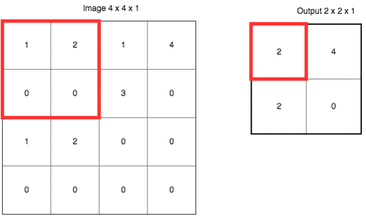
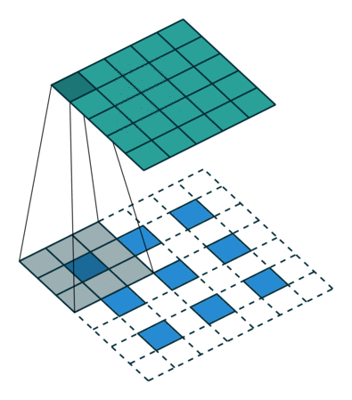
Convolution and Max Pooling Layer
Convolution layers have a lot of success with images. For this code cell, we should implement the function conv2d_maxpool to apply convolution then max pooling:
* Create the weight and bias using conv_ksize, conv_num_outputs and the shape of x_tensor.
* Apply a convolution to x_tensor using weight and conv_strides.
* We recommend you use same padding, but you’re welcome to use any padding.
* Add bias
* Add a nonlinear activation to the convolution.
* Apply Max Pooling using pool_ksize and pool_strides.
* We recommend you use same padding, but you’re welcome to use any padding.
Note: You can’t use TensorFlow Layers or TensorFlow Layers (contrib) for this layer, but you can still use TensorFlow’s Neural Network package. You may still use the shortcut option for all the other layers.
def conv2d_maxpool(x_tensor, conv_num_outputs, conv_ksize, conv_strides, pool_ksize, pool_strides):
    """
    Apply convolution then max pooling to x_tensor
    :param x_tensor: TensorFlow Tensor
    :param conv_num_outputs: Number of outputs for the convolutional layer
    :param conv_ksize: kernal size 2-D Tuple for the convolutional layer
    :param conv_strides: Stride 2-D Tuple for convolution
    :param pool_ksize: kernal size 2-D Tuple for pool
    :param pool_strides: Stride 2-D Tuple for pool
    : return: A tensor that represents convolution and max pooling of x_tensor
    """
    height = conv_ksize[0]
    width = conv_ksize[1]
    depth = x_tensor.get_shape().as_list()[3]

    weight = tf.Variable(tf.truncated_normal([height,width,depth,conv_num_outputs], stddev=0.1))
    bias = tf.Variable(tf.zeros([conv_num_outputs]))

    conv = conv = tf.nn.conv2d(x_tensor, weight, [1,conv_strides[0],conv_strides[1],1], padding='SAME')
    conv = tf.nn.bias_add(conv, bias)
    conv = tf.nn.relu(conv)
    conv = tf.nn.max_pool(
        conv,
        ksize=[1,*pool_ksize,1],
        strides=[1,*pool_strides,1],
        padding='SAME')

    return conv
Flatten Layer
Implement the flatten function to change the dimension of x_tensor from a 4-D tensor to a 2-D tensor. The output should be the shape (Batch Size, Flattened Image Size). Shortcut option: we can use classes from the TensorFlow Layers or TensorFlow Layers (contrib) packages for this layer. For more of a challenge, only use other TensorFlow packages.
def flatten(x_tensor):
    """
    Flatten x_tensor to (Batch Size, Flattened Image Size)
    : x_tensor: A tensor of size (Batch Size, ...), where ... are the image dimensions.
    : return: A tensor of size (Batch Size, Flattened Image Size).
    """

    batch_size = x_tensor.get_shape().as_list()[0]
    width  = x_tensor.get_shape().as_list()[1]
    height = x_tensor.get_shape().as_list()[2]
    depth = x_tensor.get_shape().as_list()[3]
    image_flat_size = width * height * depth

    flat = tf.contrib.layers.flatten(x_tensor,[batch_size,image_flat_size])
    return flat
Fully-Connected Layer
Implement the fully_conn function to apply a fully connected layer to x_tensor with the shape (Batch Size, num_outputs). Shortcut option: we can use classes from the TensorFlow Layers or TensorFlow Layers (contrib) packages for this layer. For more of a challenge, only use other TensorFlow packages.
def fully_conn(x_tensor, num_outputs):
    """
    Apply a fully connected layer to x_tensor using weight and bias
    : x_tensor: A 2-D tensor where the first dimension is batch size.
    : num_outputs: The number of output that the new tensor should be.
    : return: A 2-D tensor where the second dimension is num_outputs.
    """
    weight_rows = x_tensor.get_shape().as_list()[1]
    weights = tf.Variable(tf.truncated_normal((weight_rows, num_outputs), stddev=0.1))
    bias = tf.Variable(tf.zeros(num_outputs,dtype=tf.float32))


    fully = tf.matmul(x_tensor,weights)
    fully = tf.add(fully,bias)
    fully = tf.nn.relu(fully)

    return fully
Output Layer
Implement the output function to apply a fully connected layer to x_tensor with the shape (Batch Size, num_outputs). Shortcut option: we can use classes from the TensorFlow Layers or TensorFlow Layers (contrib) packages for this layer. For more of a challenge, only use other TensorFlow packages.
Note: Activation, softmax, or cross entropy should not be applied to this.
def output(x_tensor, num_outputs):
    """
    Apply a output layer to x_tensor using weight and bias
    : x_tensor: A 2-D tensor where the first dimension is batch size.
    : num_outputs: The number of output that the new tensor should be.
    : return: A 2-D tensor where the second dimension is num_outputs.
    """
    weight_rows = x_tensor.get_shape().as_list()[1]
    weights = tf.Variable(tf.truncated_normal([weight_rows, num_outputs], stddev=0.1))
    bias = tf.Variable(tf.zeros(num_outputs))
    out = tf.add(tf.matmul(x_tensor, weights), bias)
    return out
Create Convolutional Model
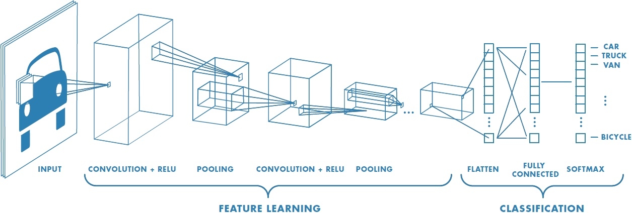
Implement the function conv_net to create a convolutional neural network model. The function takes in a batch of images, x, and outputs logits. Use the layers we created above to create this model:
- Apply 1, 2, or 3 Convolution and Max Pool layers
- Apply a Flatten Layer
- Apply 1, 2, or 3 Fully Connected Layers
- Apply an Output Layer
- Return the output
- Apply TensorFlow’s Dropout to one or more layers in the model using
keep_prob.
def conv_net(x, keep_prob):
    """
    Create a convolutional neural network model
    : x: Placeholder tensor that holds image data.
    : keep_prob: Placeholder tensor that hold dropout keep probability.
    : return: Tensor that represents logits
    """
    x_tensor = x

    conv_num_outputs1 = 64
    conv_ksize_1 = (5,5)
    conv_strides_1 = (1,1)
    pool_ksize_1 = (3,3)
    pool_strides_1 = (2,2)

    conv_num_outputs2 = 64
    conv_ksize_2 = (5,5)
    conv_strides_2 = (1,1)
    pool_ksize_2 = (3,3)
    pool_strides_2 = (2,2)

    conv = conv2d_maxpool(x_tensor, conv_num_outputs1, conv_ksize_1, conv_strides_1, pool_ksize_1, pool_strides_1)
    conv = conv2d_maxpool(conv, conv_num_outputs2, conv_ksize_2, conv_strides_2, pool_ksize_2, pool_strides_2)

    flat = flatten(conv)

    fully = fully_conn(flat, 385)
    fully = tf.nn.dropout (fully, tf.to_float(keep_prob))
    fully = fully_conn(fully, 192)

    output_data = output(fully, 10)

    return output_data

##############################
## Build the Neural Network ##
##############################

# Remove previous weights, bias, inputs, etc..
tf.reset_default_graph()

# Inputs
x = neural_net_image_input((32, 32, 3))
y = neural_net_label_input(10)
keep_prob = neural_net_keep_prob_input()

# Model
logits = conv_net(x, keep_prob)

# Name logits Tensor, so that is can be loaded from disk after training
logits = tf.identity(logits, name='logits')

# Loss and Optimizer
cost = tf.reduce_mean(tf.nn.softmax_cross_entropy_with_logits(logits=logits, labels=y))
optimizer = tf.train.AdamOptimizer().minimize(cost)

# Accuracy
correct_pred = tf.equal(tf.argmax(logits, 1), tf.argmax(y, 1))
accuracy = tf.reduce_mean(tf.cast(correct_pred, tf.float32), name='accuracy')
Neural Network Built!
Train the Neural Network
Single Optimization
Implement the function train_neural_network to do a single optimization. The optimization should use optimizer to optimize in session with a feed_dict of the following:
* x for image input
* y for labels
* keep_prob for keep probability for dropout
This function will be called for each batch, so tf.global_variables_initializer() has already been called.
Note: Nothing needs to be returned. This function is only optimizing the neural network.
def train_neural_network(session, optimizer, keep_probability, feature_batch, label_batch):
    """
    Optimize the session on a batch of images and labels
    : session: Current TensorFlow session
    : optimizer: TensorFlow optimizer function
    : keep_probability: keep probability
    : feature_batch: Batch of Numpy image data
    : label_batch: Batch of Numpy label data
    """
    feature_batch = feature_batch.astype('float32')
    label_batch = label_batch.astype('float32')
    keep_prob = neural_net_keep_prob_input()

    session.run(optimizer, feed_dict={x: feature_batch,y: label_batch,keep_prob: keep_probability})
    pass
Show Stats
Implement the function print_stats to print loss and validation accuracy. Use the global variables valid_features and valid_labels to calculate validation accuracy. Use a keep probability of 1.0 to calculate the loss and validation accuracy.
def print_stats(session, feature_batch, label_batch, cost, accuracy):
    """
    Print information about loss and validation accuracy
    : session: Current TensorFlow session
    : feature_batch: Batch of Numpy image data
    : label_batch: Batch of Numpy label data
    : cost: TensorFlow cost function
    : accuracy: TensorFlow accuracy function
    """
    loss = session.run(cost, feed_dict =
                   {x: feature_batch,y: label_batch, keep_prob: 1.0})
    acc = session.run(accuracy,feed_dict =
                  {x: valid_features, y: valid_labels, keep_prob: 1.0})
    print('Loss at {}'.format(loss), 'Validation Accuracy at {}'.format(acc))
    pass
Hyperparameters
Tune the following parameters:
* Set epochs to the number of iterations until the network stops learning or start overfitting
* Set batch_size to the highest number that our machine has memory for. Most people set them to common sizes of memory:
* 64
* 128
* 256
* …
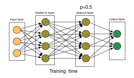
* Set keep_probability to the probability of keeping a node using dropout

# Tune Parameters
epochs = 3
batch_size = 64
keep_probability = 0.75
Train on a Single CIFAR-10 Batch
Instead of training the neural network on all the CIFAR-10 batches of data, let’s use a single batch. This should save time while we iterate on the model to get a better accuracy. Once the final validation accuracy is 50% or greater, run the model on all the data in the next section.
print('Checking the Training on a Single Batch...')
with tf.Session() as sess:
    # Initializing the variables
    sess.run(tf.global_variables_initializer())

    # Training cycle
    for epoch in range(epochs):
        batch_i = 1
        for batch_features, batch_labels in helper.load_preprocess_training_batch(batch_i, batch_size):
            train_neural_network(sess, optimizer, keep_probability, batch_features, batch_labels)
        print('Epoch {:>2}, CIFAR-10 Batch {}:  '.format(epoch + 1, batch_i), end='')
        print_stats(sess, batch_features, batch_labels, cost, accuracy)
Checking the Training on a Single Batch...
Epoch  1, CIFAR-10 Batch 1:  Loss at 1.815567970275879 Validation Accuracy at 0.4291999936103821
Epoch  2, CIFAR-10 Batch 1:  Loss at 1.6947548389434814 Validation Accuracy at 0.43880000710487366
Epoch  3, CIFAR-10 Batch 1:  Loss at 1.4058599472045898 Validation Accuracy at 0.4675999879837036
Fully Train the Model
Now that we got a good accuracy with a single CIFAR-10 batch, try it with all five batches.
#Tune Parameters
epochs = 2
batch_size = 64
keep_probability = 0.75
save_model_path = './image_classification'

print('Training...')
with tf.Session() as sess:
    # Initializing the variables
    sess.run(tf.global_variables_initializer())

    # Training cycle
    for epoch in range(epochs):
        # Loop over all batches
        n_batches = 5
        for batch_i in range(1, n_batches + 1):
            for batch_features, batch_labels in helper.load_preprocess_training_batch(batch_i, batch_size):
                train_neural_network(sess, optimizer, keep_probability, batch_features, batch_labels)
            print('Epoch {:>2}, CIFAR-10 Batch {}:  '.format(epoch + 1, batch_i), end='')
            print_stats(sess, batch_features, batch_labels, cost, accuracy)

    # Save Model
    saver = tf.train.Saver()
    save_path = saver.save(sess, save_model_path)
Training...
Epoch  1, CIFAR-10 Batch 1:  Loss at 1.8637771606445312 Validation Accuracy at 0.37459999322891235
Epoch  1, CIFAR-10 Batch 2:  Loss at 1.490159273147583 Validation Accuracy at 0.46459999680519104
Epoch  1, CIFAR-10 Batch 3:  Loss at 1.2188395261764526 Validation Accuracy at 0.5059999823570251
Epoch  1, CIFAR-10 Batch 4:  Loss at 1.1865193843841553 Validation Accuracy at 0.5383999943733215
Epoch  1, CIFAR-10 Batch 5:  Loss at 1.1775325536727905 Validation Accuracy at 0.5302000045776367
Epoch  2, CIFAR-10 Batch 1:  Loss at 1.3255388736724854 Validation Accuracy at 0.5508000254631042
Epoch  2, CIFAR-10 Batch 2:  Loss at 1.0641307830810547 Validation Accuracy at 0.5547999739646912
Epoch  2, CIFAR-10 Batch 3:  Loss at 0.9235615730285645 Validation Accuracy at 0.5928000211715698
Epoch  2, CIFAR-10 Batch 4:  Loss at 0.8957799673080444 Validation Accuracy at 0.605400025844574
Epoch  2, CIFAR-10 Batch 5:  Loss at 0.8781595230102539 Validation Accuracy at 0.6154000163078308
Checkpoint
The model has been saved to disk.
Test Model
Test our model against the test dataset. This will be our final accuracy. We should have an accuracy greater than 50%. If we don’t, we need keep tweaking the model architecture and parameters.
%matplotlib inline
%config InlineBackend.figure_format = 'retina'
import tensorflow as tf
import pickle
import helper
import random
# Set batch size if not already set
try:
if batch_size:
pass
except NameError:
batch_size = 64
save_model_path = './image_classification'
n_samples = 4
top_n_predictions = 3
def test_model():
"""
Test the saved model against the test dataset
"""
test_features, test_labels = pickle.load(open('preprocess_training.p', mode='rb'))
loaded_graph = tf.Graph()
with tf.Session(graph=loaded_graph) as sess:
# Load model
loader = tf.train.import_meta_graph(save_model_path + '.meta')
loader.restore(sess, save_model_path)
# Get Tensors from loaded model
loaded_x = loaded_graph.get_tensor_by_name('x:0')
loaded_y = loaded_graph.get_tensor_by_name('y:0')
loaded_keep_prob = loaded_graph.get_tensor_by_name('keep_prob:0')
loaded_logits = loaded_graph.get_tensor_by_name('logits:0')
loaded_acc = loaded_graph.get_tensor_by_name('accuracy:0')
# Get accuracy in batches for memory limitations
test_batch_acc_total = 0
test_batch_count = 0
for train_feature_batch, train_label_batch in helper.batch_features_labels(test_features, test_labels, batch_size):
test_batch_acc_total += sess.run(
loaded_acc,
feed_dict={loaded_x: train_feature_batch, loaded_y: train_label_batch, loaded_keep_prob: 1.0})
test_batch_count += 1
print('Testing Accuracy: {}\n'.format(test_batch_acc_total/test_batch_count))
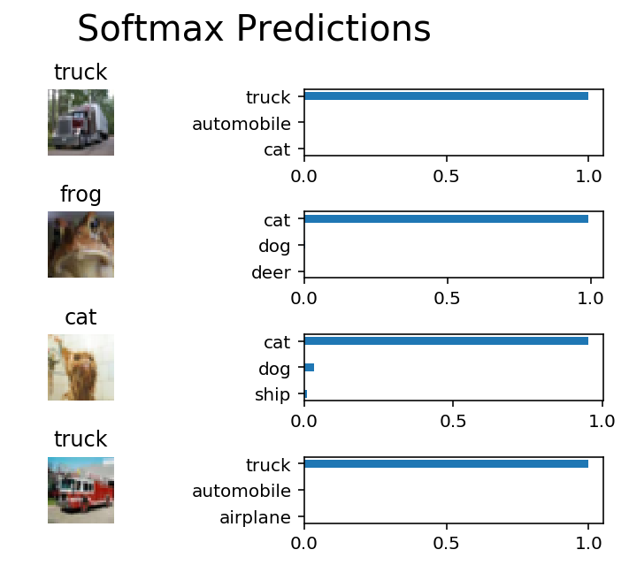
# Print Random Samples
random_test_features, random_test_labels = tuple(zip(*random.sample(list(zip(test_features, test_labels)), n_samples)))
random_test_predictions = sess.run(
tf.nn.top_k(tf.nn.softmax(loaded_logits), top_n_predictions),
feed_dict={loaded_x: random_test_features, loaded_y: random_test_labels, loaded_keep_prob: 1.0})
helper.display_image_predictions(random_test_features, random_test_labels, random_test_predictions)
test_model()
Testing Accuracy: 0.71806640625
Why 50-80% Accuracy?
You might be wondering why we can’t get an accuracy any higher. First things first, 50% isn’t bad for a simple CNN. Pure guessing would get you 10% accuracy. However, you might notice people are getting scores well above 80%. That’s because we need to cover a few more techniques.